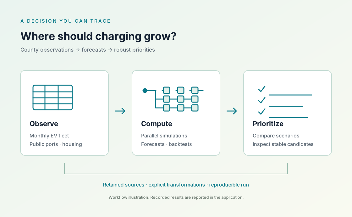
Turn government EV registrations and public charging records into a shortlist for investment. Forecast county adoption, inspect charging pressure, and see which priorities survive different assumptions.
One scientific workflow: collect observations, make the transformations explicit, compare forecasts, and inspect a decision under uncertainty.
Study snapshot: retrieved 2026-10-28 · observations through 2026-09. 39 Washington counties; passenger and truck BEV + PHEV registrations. The current charging inventory and ACS 2020–2024 housing estimates have different observation dates.
START WITH THE DECISION
Three questions a planning team can use.
Washington provides a monthly registration history and a clear geographic unit: the county. This case connects a reproducible forecast to an initial infrastructure screening decision.
01 / ADOPTION
How much could the EV fleet grow in the next 12 months?
Compare a recent trend forecast with a last observed value baseline using past forecast cutoffs. Report the error before interpreting the projection.
Decision: plan the scale and timing of further charging assessment.
02 / INFRASTRUCTURE
Where is the projected EV fleet large relative to today’s public ports?
Combine county projections with a dated inventory of public charging ports. Keep Level 2 and DC fast charging counts visible so their different roles remain clear.
Decision: identify counties for a closer study of sites, access and capacity.
03 / ROBUSTNESS
Which priorities persist when the assumptions change?
Repeat the screening under slower and faster adoption, then introduce renter share as an explicit sensitivity rule. Inspect changes in the shortlist.
Decision: distinguish stable candidates from places whose priority depends on a chosen rule.
EVIDENCE BEFORE RECOMMENDATION
What the recorded run tells us.
These are results for the retained data snapshot and declared assumptions. County screening supports the next planning decision; a final site requires local evidence about electricity capacity, road access, utilization and cost.
Observed EV fleet291,499
Registered BEVs and plug-in hybrids, September 2026.
Conditional 12-month projection≈332,800
14.2% above observed stock; 24-month drift through September 2027.
Lower historical forecast error67.9%
County macro-average MAE against persistence, across 12 rolling origins.
Listed public charging ports6,739 L2 · 2,428 DC
3,225 public sites listed as available, October 28, 2026.
01 / A useful baseline beats no growth
The 24-month drift projects approximately 332,800 registered EVs in September 2027, from 291,499. Mean county absolute error at a 12-month horizon is 357.7 vehicles, against 1,113.1 for persistence; drift performs better in 38 of 39 counties. The projection assumes recent net registration changes remain representative.
02 / Fleet size does not determine pressure
Douglas, Cowlitz and Snohomish lead the projected EVs per Level 2 port screen. Douglas has 4 listed public Level 2 ports against a conditional fleet projection of 820 EVs. Garfield has no listed public Level 2 ports and requires separate investigation; assigning it an artificial denominator would hide that gap.
03 / Six counties remain on the shortlist
Douglas, Cowlitz, Snohomish, Kitsap, Grant and Thurston remain in the top 10 under all nine combinations of adoption and renter weighting. These stable candidates warrant local assessment. Wahkiakum appears in only three scenarios, illustrating how priorities can depend on the selected equity rule.
Teal: observed stock. Orange: forecast. Recent observed fleet totals and the conditional drift projection. The orange line interpolates the 12-month endpoint under a constant net increase assumption; it is not a probability interval.
Forecast validation on observations held out in time. Lower mean absolute error is better; errors are measured in registered vehicles.
Method
Mean absolute error
Evaluation
24-month drift
357.7
County macro-average; 12 rolling origins and a 12-month horizon.
Persistence
1,113.1
Predict unchanged stock from each historical origin.
Validation uses 12 historical origins, October 2024–September 2025, each with the preceding 24 monthly changes and a 12-month target held out in time. The table reports the average of county mean absolute errors, not a statewide total error. The forecast horizons overlap, so the errors are not independent replicates.
The top 10 counties by projected EVs per currently listed public Level 2 port. DC fast inventory is shown separately; BEV + PHEV stock does not measure DC-compatible demand.
County
Observed EVs
Projected EVs
Level 2 ports
DC fast ports
EVs / Level 2 port
Renter share
Top 10 scenarios
Douglas
697
820
4
9
205
30.7%
9 / 9
Cowlitz
1,683
1,967
12
26
163.9
32%
9 / 9
Snohomish
37,252
43,033
307
300
140.2
31.8%
9 / 9
Wahkiakum
107
124
1
1
124
16.8%
3 / 9
Mason
1,602
1,902
18
0
105.7
17.7%
3 / 9
Lewis
1,431
1,669
16
60
104.3
24.2%
6 / 9
Kitsap
10,080
11,657
133
83
87.6
29.9%
9 / 9
Island
3,254
3,757
44
6
85.4
25.3%
3 / 9
Grant
1,282
1,552
21
45
73.9
33.7%
9 / 9
Thurston
9,785
11,308
167
129
67.7
32.3%
9 / 9
The sensitivity rule is part of the decision.
Rank 38 counties with positive Level 2 counts under nine combinations: scale the forecast net increase by 0.75, 1 or 1.25, then apply renter weights of 0, 0.25 or 0.5.
Midrank percentiles normalize the two indicators; tied final scores use ascending county FIPS. Garfield’s zero Level 2 count is flagged separately. The shared growth settings leave top-ten membership and order unchanged at each renter weight, so the nine combinations produce three distinct shortlist rankings. Weights express planning preferences, and ACS uncertainty is not propagated into rank confidence intervals.
EVs per public Level 2 port is a screening indicator. County boundaries hide travel across counties, and registered vehicles do not measure charging sessions. Renter share provides context about potential home charging constraints; it does not measure an individual household’s access. Forty-eight retained public station listings have restricted-access flags, so this inventory does not imply unrestricted, round-the-clock service.
WHY THESE COUNTIES?
Change the assumptions. Inspect the recommendation.
Choose a county to follow its registered fleet, forecast, station records and housing context. The six stable candidates remain in the top ten within the tested settings; Kitsap is closer to the cutoff, while Wahkiakum shows how a different weighting can change the shortlist.
Six candidates that remain in the top ten, plus Wahkiakum for comparison. Ranks compare 38 counties with positive listed L2 counts.
Select county
Projected EVs / L2 port
Renter share
Selected rank
Rank range
205
30.7%
1
1–2
163.9
32%
2
1–2
140.2
31.8%
3
3–4
87.6
29.9%
7
5–10
73.9
33.7%
9
4–9
67.7
32.3%
10
7–10
124
16.8%
4
4–22
The nine settings produce three distinct top-ten rankings. In this tested range, changing the shared growth multiplier changes pressure values but leaves each top-ten membership and order unchanged. “Top ten in 9/9” describes stability within these assumptions; it is not a confidence probability.
COUNTY FIPS 53017
Douglas: follow the recommendation.
9 / 9settings in the top ten
The strongest L2 pressure indicator keeps Douglas first or second. Its small listed inventory is the main reason to investigate access locally; renter context keeps it competitive as the weighting changes.
At 1.00 × growth and 0% renter weight, Douglas ranks 1 of 38 with 205 projected EVs per listed L2 port.
01 / OBSERVATIONS
Retain the county’s fleet history.
DOL registered EV stock: 451 in September 2024 → 697 in September 2026. Passenger and Truck rows include BEVs and plug-in hybrids.
4 listed L2 ports across 4 L2 station records. DC fast ports are recorded separately: 9. ACS renter-occupied units: 4,892 / 15,923 = 30.72%.
ACS 2020–2024 source margins of error, at 90% confidence: ±440 renter units and ±330 occupied units. The ranking does not propagate these into rank confidence intervals.
Pressure contributes 1.000 and renter context contributes 0.000 to the score. Both indicators are converted to midrank percentiles before weighting. Final ties use ascending county FIPS.
Verify Douglas’s Level 2 station records · 4 records / 4 ports
These are the AFDC IDs assigned to this county by the retained point-to-county join. Listed availability and public access do not establish measured uptime or unrestricted service.
The runnable case starts from curated government CSV snapshots. Aner performs the forecasts, historical evaluation, repeated uncertainty calculations, scenario ranking and maps, with the execution policy visible.
Repeat the forecast with a declared seed.
Independent simulations give a natural boundary for local parallelism. Each repetition uses its own random stream, and ordered results make a serial comparison possible.
The same task can use a configured cluster. The optional cluster route requires matching runtimes and enrolled workers; this case reports distributed performance only when that execution has actually been measured.
// initial and changes retain this county’s observation history.let execution = parallel.local(workers: 4)
let paths = parallel.repeat(iterations: 1000, task: bootstrap_stock,
parameters: List(initial, changes), execution: execution, seed: 20261028 + county_index,
max_bytes: 1048576)
paths.save_csv("generated/bootstrap-" + fips + ".csv")
Recorded execution: 1,000 repetitions per county · 39 counties · 4 local workers
Base seed 20261028; county offsets are retained. All 39,000 ordered bootstrap paths and county results were byte-identical with one and four workers. The repository also provides an optional cluster route; a multi-computer performance comparison remains a separate experiment.
The 10th–90th bootstrap percentiles are assumption-based ranges. Their coverage has not been calibrated against future observations.
Put observations on the map.
Use Aner Plot to inspect station locations and county context. Port counts, station locations and geographic boundaries retain their source dates alongside the chart.
A station marker describes a reported location. It does not establish opening hours, current uptime or vehicle compatibility.
// positions, ports and labels come from the retained station records.let boundaries = plot.geojson("data/wa-counties.geojson")
let chart = plot.choropleth(geojson: boundaries, property: "GEOID",
keys: List(), values: List())
.add_points(positions: positions, values: ports, labels: labels)
.point_sizes(values: ports, max_radius: 7.0)
.point_labels("none")
.extent(west: -124.9, south: 45.4, east: -116.8, north: 49.1)
.projection("lambert_azimuthal_equal_area")
.annotate(x: -121.8360321, y: 47.4908756, text: "King County")
.annotate(x: -119.6934396, y: 47.7357217, text: "Douglas County")
.size(width: 1200, height: 780)
.theme(plot.theme("light"))
.title("Washington public EV charging")
.caption("AFDC inventory: 28 Oct 2026. Boundaries: U.S. Census 2025, shoreline-clipped cartographic display. Circle area = listed L2 + DC ports; inventory is not interchangeable capacity or measured use. County fill is context only.")
chart.save("generated/stations.svg")
// Native SVG/HTML exports are static. The website adds browser map controls.
chart.save("generated/stations.html")
Native Aner Plot output uses retained 2025 Census cartographic county geometry and 3,224 sites with positive combined port counts. One zero-port listing is omitted. Combined port counts describe inventory, not interchangeable charging capacity.
The case retains the downloaded bytes, the rules used to transform them, the parameters used in computation, and the output of the native run. A forecast can be reviewed and reproduced against its original snapshot.
01 / COLLECT
Retain the source.
Record the exact query, retrieval time, source identity and SHA-256 of each raw download. A changing government portal does not silently replace the retained evidence.
02 / TRANSFORM
Make every join explicit.
Declare county identifiers, dates, EV definitions and public access filters. Keep unmatched records, exclusions and missing values visible in the quality report.
03 / COMPUTE
Keep the experiment.
Retain forecast cutoffs, scenario assumptions, seeds, execution receipts and the runtime identity. Hold future observations out of past forecast fits.
04 / INTERPRET
Trace the decision.
Save each county’s inputs and outputs, then compare the shortlist across scenarios. Separate observed counts, model estimates and planning assumptions.
A COMPLETE WORKED TRACE
Douglas County: from observations to a shortlist.
The same county key, 53017, connects the source records, native computation and ranked output. The explorer above exposes this path for each displayed county.
Read the observations. DOL records 432 Passenger + 19 Truck EVs in September 2024, then 661 + 36 in September 2026. The prepared county totals are 451 and 697. Inspect the monthly inputs.
Compute the conditional forecast in Aner. The retained native function gives 697 + 0.5 × (697 − 451) = 820. Read ev_charging.aner.
Verify the denominator and context. AFDC IDs 63444, 262727, 262728 and 262737 each contribute one L2 port: 820 / 4 = 205 projected EVs per port. ACS table B25003 supplies 4,892 renter units out of 15,923 occupied units. Check the county join and the ACS cells.
Apply the declared preference rule in Aner. At a 25% renter weight, Douglas contributes 0.75 × 1.000 + 0.25 × 0.595 ≈ 0.899. It ranks first; at a 50% renter weight, Cowlitz moves ahead. Read county_priorities.aner.
The base seed is 20261028 with a retained county offset. Douglas uses seed 20261036 and sample file bootstrap-53017.csv. The native receipts and run manifest bind the calculations to their source tables and exact code.
Traceability comes from the complete retained workflow. Native execution receipts describe Aner’s computation; the accompanying manifest records external downloads and study choices.
Start with county forecasting and infrastructure screening, where the evidence can answer the question. Use policy and environmental records to explain context and define further studies.
Monthly registered fleet counts support a temporal adoption study. This snapshot aggregates BEVs and plug-in hybrids across passenger vehicles and trucks.
39 counties · January 2017–September 2026 · 4,563 county-month observations. A vehicle’s model year is not its registration date.
“Income and racial disparity in household publicly available electric vehicle infrastructure accessibility” motivates looking beyond infrastructure totals to household access.
Nature Communications 15, 5106 (2024), open access. Research informs the screening design; it does not validate a new county ranking.
“Analytic Tools for Locating, Sizing, and Evaluating Electric Vehicle Charging Stations” provides a Washington planning reference for forecasting and DC fast charging demand.
WA-RD 930.1 (June 2023), open report. Read alongside the assumptions and geographic resolution of this application.
INSPECT · REPRODUCE · EXTEND
Keep the code with the evidence.
Explore the Aner programs, curated CSV inputs, source records and retained native evidence on GitHub. Run the analysis from the frozen snapshot and inspect how each recommendation was produced. The executable code is supplied as .aner or .anernb files.