
Heat diffusion with uncertain parameters
Run independent transient heat diffusion realizations with heterogeneous material coefficients and uncertain source amplitude, then interpret numerical stability, output distributions and Monte Carlo sampling error.
This worked research example estimates how uncertain material diffusivity and heat source amplitude change the temperature response of a one dimensional rod. It runs 1,000 independent transient realizations, each starting from the same temperature field and boundary conditions, and retains four observables per realization. The model is a complete numerical experiment with explicit assumptions and synthetic inputs.
The guide belongs to aner.parallel. Import aner.parallel; there is no heat diffusion submodule. Use the repetition API for the checked named task contract, private input copies, RNG, resource limits, result accessors and diagnostics.
Run the complete study
Open the runnable heat diffusion example for the source and run commands, or download the complete heat diffusion source and use an updated native Aner executable:
aner check examples/parallel/repeat_heat_diffusion.aner
aner examples/parallel/repeat_heat_diffusion.aner --max-steps 5000000
The source explicitly requests four workers and requires at least four admitted CPU slots. The published run command explicitly sets --max-steps 5000000 as a reproducible per task interpreter budget with headroom for refinement. The current 31 point, 400 step fixture also fits the default budget; increasing grid size or step count may require adjusting it. The execution budget is not a time limit, physical time step or numerical stability setting. parallel.inventory() describes the discovered allocation. Checking performs no realizations. Running performs 1,000 realizations with 31 grid points and 400 time steps each, then serial output analysis. No external dataset, network, service or credential is required. The optional CSV export is commented, so a normal run creates no file. VS Code extension 0.1.39 provides the compatible task and result help.
Experiment configuration
HeatExperiment is a user defined class with eleven public, immutable scalar fields. One checked instance is wrapped in List(checked.unwrap()) and supplied to every realization. Its values are explicitly declared by the source:
| Field | Default | Meaning and units |
|---|---|---|
points: Int64 | 31 | Odd grid point count including both boundary points; at least 3. |
length_m: Float64 | 0.1 | Rod length in m; positive. |
dt_s: Float64 | 0.1 | Explicit time step in s; positive and subject to the CFL bound. |
steps: Int64 | 400 | Positive update count; final time is steps × dt_s = 40 s. |
pulse_steps: Int64 | 200 | Heating steps, from 0 through steps; pulse duration is pulse_steps × dt_s = 20 s. |
ambient_k: Float64 | 293.15 | Positive common initial and fixed endpoint temperature in K. |
diffusivity_m2_s: Float64 | 0.00001 | Nominal thermal diffusivity in m²/s; positive. |
diffusivity_spread: Float64 | 0.25 | Dimensionless relative half width of the uniform face uncertainty; from 0 up to, excluding, 1. |
source_k_s: Float64 | 3.0 | Nominal temperature rise rate in K/s within the heater; nonnegative. |
source_spread: Float64 | 0.2 | Dimensionless relative half width of source amplitude uncertainty; from 0 through 1. |
threshold_k: Float64 | 335.0 | Positive K threshold for the global peak exceedance indicator. |
validate_experiment(c: HeatExperiment) -> Result<HeatExperiment, String> checks finite Float64 inputs, these ranges, finite positive derived spatial quantities, and the worst case diffusion stability bound. Serial setup prints a validation error and .unwrap() stops an invalid experiment. The checked task repeats validation for its private copied instance. Use finite scalar settings and update the output labels when changing the declared threshold. For Result construction, inspection and checked payload access, see the Result reference.
This fragment belongs to the complete source, which declares heat_realization and initial_parameters:
let results = parallel.repeat(iterations: 1000, task: heat_realization,
    parameters: initial_parameters,
    execution: parallel.local(workers: 4), seed: 2026)
The BEGIN PARALLEL and END PARALLEL comments surround this call; the call selects the execution policy. Setup and later analysis remain serial. Each realization gets the same nominal HeatExperiment; its seed selects a different material and source realization.
Physical and uncertainty model
Let T(x,t) be temperature in kelvin and α(x) the thermal diffusivity in m²/s. The modeled temperature equation is:
∂T/∂t = ∂/∂x [ α(x) ∂T/∂x ] + s(x,t)The source s is a temperature rise rate in K/s. It represents volumetric heating already divided by a constant volumetric heat capacity. Thermal diffusivity is distinct from conductivity; converting an experimental power density or thermal conductivity into these inputs requires consistent density and heat capacity assumptions.
The rod is 0.1 m long. Its 31 grid points include both ends, giving 30 intervals and spacing Δx = 0.1/30 m. Every realization starts with T = 293.15 K at all points. Both ends remain fixed at 293.15 K throughout the run: these are Dirichlet boundary conditions representing ideal temperature reservoirs. The study advances 400 steps of Δt = 0.1 s, covering 40 s. A heating pulse operates during the first 20 s, followed by 20 s of cooling and diffusion.
For each face f, the source uses α_f = α₀ × (1 + 0.25 × (2 U_f − 1)), with a uniform simulation draw U_f in [0,1). The default face diffusivities therefore lie from 7.5 × 10⁻⁶ up to, excluding, 1.25 × 10⁻⁵ m²/s. Draw identities 0 through 29 address the 30 faces. One separate draw at identity 30 selects an amplitude multiplier A = 1 + 0.2 × (2 U₃₀ − 1), giving a heater rate from 2.4 up to, excluding, 3.6 K/s. Both the face values and amplitude stay fixed through all 400 steps of a realization.
The heater covers the central third of the rod, x ∈ [L/3, 2L/3]. Its source is averaged over each interior node’s control volume of width Δx: the fraction is the length overlapping that heater divided by Δx. On the default grid, nodes 10 and 20 receive half strength, nodes 11 through 19 receive full strength, and other nodes receive zero. This preserves the central third heating integral on this grid. Heating is active at step indices 0 through 199; step 200 begins the source free part of the 40 s horizon.
The random field models fixed spatial heterogeneity, rather than fresh temporal noise. All realizations use the same sampling rule and common initial field. These bounded uniform uncertainties are synthetic assumptions, which must be replaced or justified when modeling a measured material.
Conservative spatial update and explicit time stepping
At each interior point, the update uses fluxes across its left and right faces. With i a spatial index and n a time step index:
Tᵢⁿ⁺¹ = Tᵢⁿ + Δt/Δx² × [
    αᵢ₊½ (Tᵢ₊₁ⁿ − Tᵢⁿ) − αᵢ₋½ (Tᵢⁿ − Tᵢ₋₁ⁿ)
] + Δt × sᵢⁿ
Using the same face coefficient for adjacent control volumes makes their shared flux contributions cancel in the interior sum. This is the conservative flux difference form of the heterogeneous diffusion term; the face based diffusion derivation is described in NIST’s finite volume discretization reference. It is not interchangeable with multiplying an ordinary second difference by an arbitrary cell centered diffusivity when the coefficient varies spatially.
The source reads every right hand side temperature from the current time layer and writes a separate next layer. Both buffers retain their initially fixed endpoint values, because the update writes only interior entries before swapping the buffers. In place updates would mix time layers and implement a different numerical scheme. The source is evaluated at the current step time; the temperature update is explicit forward Euler.
CFL stability bound
For nonnegative diffusivities, a sufficient diffusion CFL condition for this explicit update is:
Δt × (αᵢ₋½ + αᵢ₊½) / Δx² ≤ 1 for every interior pointUnder this condition the diffusion only update is a convex combination of current neighboring temperatures. The stronger convenient bound 2 α_max Δt / Δx² ≤ 1 accounts for the largest allowed diffusivity, including the uncertainty range. With the defaults, α_max = 1.25 × 10⁻⁵ m²/s, Δx = 1/300 m and Δt = 0.1 s, the bound is 0.225, below 1. The source validator rejects settings above 1 before entering the executor. The additive prescribed heat source changes temperature without changing those diffusion weights.
For constant diffusivity this reduces to R = α Δt/Δx² ≤ 1/2, the explicit heat equation stability condition discussed in Gilbert Strang’s MIT numerical methods notes, printed page 205. The heterogeneous bound above follows from requiring every coefficient in this source’s diffusion update to be nonnegative.
Recalculate the bound whenever the grid spacing, time step, nominal diffusivity or uncertainty interval changes. Refining the grid by a factor of two generally requires reducing an explicit diffusion time step by a factor of four to retain the same bound. Satisfying the CFL limit establishes this numerical stability condition; it does not establish spatial/time step accuracy or physical model validity.
Parallel execution and reproducibility
Serial setup constructs one initial parameter List. Only the parallel.repeat call runs on the local executor. A checked task privately creates and evolves one realization's temperature buffers and material coefficients, then returns one four value List. No temperature field is shared between realizations. Its 400 dependent time steps run in order inside the task; the executor distributes independent realizations across workers.
The supplied task seed derives from the master seed and zero based realization index. The source uses parallel.random(seed, draw: face) for each material face and draw: points − 1 for the separate source amplitude. Worker count and completion order do not change those identities or result row ordering. Preserve the source, native build, parameters and master seed when comparing runs. The generator is for reproducible simulation, rather than cryptographic use; deterministic draw separation is not evidence that a proposed physical covariance model is valid.
Setup, printing, statistics and optional export occur on the caller after every result row is complete. Unsupported task effects or captures produce E2803; runtime task, result, budget and accessor failures use R2803. No successful partial batch is published. The checked task and SimulationResults API are the same as in the repetition reference.
Output observables and statistics
Results contain 1,000 ordered rows and four Float64 columns:
| Column | Observable | Definition and units |
|---|---|---|
| 0 | Global peak temperature | Largest temperature over every grid point and every update, including the initial ambient value; K. |
| 1 | Final center temperature | Temperature at index points/2, at 40 s for the defaults; K. |
| 2 | Final spatial mean temperature | Trapezoidal length average of the final rod profile, with half endpoint weights; K. |
| 3 | Threshold indicator | 1.0 if the global peak is strictly greater than 335.0 K, otherwise 0.0; dimensionless. |
Both endpoints equal ambient_k, so the trapezoidal mean simplifies to (temperature.sum() − ambient_k)/(points − 1). It includes the boundaries with their half weights and is not an equal point arithmetic mean. The indicator uses strict >: equality with the threshold does not count as exceedance. Preserve this column interpretation when exporting data; the generic CSV headers do not encode physical units.
results.mean(column: c) summarizes an observable across realizations. results.std(column: c, sample: true) estimates the spread of those model outputs using denominator N − 1. That spread describes variation from the specified uncertain inputs. It is distinct from Monte Carlo uncertainty in the estimated ensemble mean.
For N = 1000, the usual independent realization estimate of the mean's standard error is:
standard error of estimated mean = sample standard deviation / sqrt(N)The threshold indicator's mean estimates an exceedance probability, p_hat = exceedance_count/N. A binomial Monte Carlo standard error is sqrt(p_hat × (1 − p_hat)/N). This plug in estimate can be zero when every sampled outcome lies on the same side of the threshold; that does not prove the true probability is exactly zero or one.
The complete source also prints an approximate 95% Wilson interval using z = 1.96, following the NIST proportion interval formulation:
denominator = 1 + z²/N
center = (p_hat + z²/(2N)) / denominator
half_width = z × sqrt(p_hat(1−p_hat)/N + z²/(4N²)) / denominator
interval = [center − half_width, center + half_width]
This interval describes Monte Carlo uncertainty in the exceedance probability under the specified sampling model. It is distinct from the physical output spread and from uncertainty about the model's assumptions. Rare event estimates can require substantially more realizations. The source's probability_root helper uses 40 Newton steps for these bounded nonnegative probability expressions at N = 1000; it is a local teaching helper, not a general square root API.
Temperature spread, standard error, and threshold probability answer different questions. Increasing the realization count reduces Monte Carlo error under the stated sampling assumptions; it does not repair a spatial discretization error, a coarse time step or an unsupported uncertainty distribution. Retain the output rows to study tails and associations among observables, rather than keeping only averages.
Read and export the completed results
The program prints the realization count, peak temperature mean and sample standard deviation, final center mean, final spatial mean temperature, peak exceedance fraction, its Monte Carlo standard error and Wilson interval, and native executor seconds. The first line is Independent realizations: 1000. The statistics depend on the declared inputs and seeded source; executor seconds also depend on the machine and competing work.
A verified run with the default configuration and master seed 2026 produced these rounded reference values:
| Printed statistic | Reference result |
|---|---|
| Peak temperature mean | 340.4654 K |
| Peak temperature sample standard deviation | 5.5471 K |
| Final center temperature mean | 323.9687 K |
| Final spatial mean temperature | 310.9217 K |
| Fraction of peaks strictly above 335 K | 0.777, or 777 of 1,000 realizations |
| Monte Carlo probability standard error | 0.01316 |
| Approximate 95% Wilson interval | 0.7502 to 0.8017 |
These are seeded synthetic model outputs. They are a reproducible reference for this configuration, rather than empirical material measurements or a performance benchmark. Floating point details can depend on the native build; executor time is deliberately omitted from this numerical reference.
After the repeat call, these supported accessors inspect the retained observables:
print(results.value(iteration: 0, column: 0))
print(results.mean(column: 1))
print(results.std(column: 0, sample: true))
print(results.seed(iteration: 0))
These lines are an optional fragment after results is created by the complete program. Keep full row/column identities when investigating correlations and tails. If export is needed, uncomment results.save_csv("heat-realizations.csv") only with a new destination. Its parent directory must already exist; the API refuses an existing path. The header is iteration,seed,value_0,value_1,value_2,value_3, with precise Float64 values and exact decimal seeds. See CSV ownership and lifecycle for the full export contract.
Measured numerical verification
A separate homogeneous verification variant used the initial temperature profile T(x,0) = 293.15 + 10 sin(πx/L), in K, uniform diffusivity α = 10⁻⁵ m²/s, no heating, L = 0.1 m and fixed 293.15 K endpoints. It compares against the exact continuum solution T(x,t) = 293.15 + 10 sin(πx/L) exp(−α(π/L)²t). This variant tests the numerical method; the default ensemble instead starts uniformly at ambient temperature and samples heterogeneous faces and a heating amplitude.
All three refinements cover 40 s and keep R = α Δt/Δx² = 0.09:
| Grid points | Time step (s) | Updates | Maximum nodal error against continuum (K) | Error reduction |
|---|---|---|---|---|
| 31 | 0.1 | 400 | 0.0011189950624 | Baseline |
| 61 | 0.025 | 1,600 | 0.0002796100603 | 4.00198× |
| 121 | 0.00625 | 6,400 | 0.0000698938471 | 4.00050× |
Every final node also agrees with the exact discrete sine mode amplification solution within 3.42 × 10⁻¹³ K. The approximately fourfold error reduction is the measured behavior of this homogeneous test with space and time refined together; it does not establish convergence for a stochastic face field redrawn on every new grid.
Additional recorded checks found exact output row and derived seed equality for an instrumented eight realization cohort on one and four workers. Source free uniform fields remained exactly 293.15 K; fixed endpoints, temperature bounds and post pulse maximum decay had no violations. The integrated temperature update balanced the source and boundary flux to within 1.135 × 10⁻¹⁴ K·m. All 19 invalid configuration cases were rejected, including unstable steps, invalid ranges, NaN, infinity and extreme lengths. These are numerical and implementation checks, with no performance claim or experimental material validation.
Numerical checks and research limitations
Before using the experiment for a research conclusion, validate several separate parts:
- Check baseline and limiting cases: zero heating with a uniform initial field and fixed equal boundaries should preserve the baseline temperature; zero uncertainty should give the same deterministic observables in every realization.
- Compare one and four admitted workers using the same source, parameters and master seed, then check all output rows and seeds before interpreting timings.
- Perform spatial and temporal convergence studies on the observables, maintaining the CFL bound when the grid is refined. Hold the uncertain physical input definition constant; independently resampling a different sized face field changes that definition.
- Justify the uncertainty distributions and spatial correlations from the research problem. Independent face values at a chosen grid resolution do not specify a mesh independent material field.
The model assumes one spatial dimension, a fixed geometry, prescribed source shape, constant effective volumetric heat capacity and boundary reservoirs. It omits radiation, convection, temperature dependent properties, phase change and feedback. Those effects require a revised equation, discretization and validation. This example carries scalar units in its documented model; it does not automatically enforce them through a scientific unit type.
Work, storage and timing
For N realizations, G grid points, S time steps and P admitted workers, interior evolution requires O(N S G) arithmetic work and O(P G) active field storage, plus private parameter copies and the runtime's bounded interpreter state. Four observables retain O(4 N) numeric storage. The 1,000 × 4 Float64 payload is 32,000 bytes; completion flags, allocated capacity and fixed/runtime overhead remain separate parts of native accounting. The default 64 MiB result budget is not a total process memory quota.
Read results.seconds() and results.summary() for the admitted allocation and native executor timing. That timing includes task evaluation, per realization copying and row commits; it excludes initial admission/snapshot, context startup, final publication, statistics and CSV export. Record separate whole source wall time for end to end comparisons. More arithmetic per task can amortize scheduling cost, but measured speedup still depends on allocation, implementation and competing work.
Measured 10,000 realization CPU benchmark
The complete heat benchmark runs 10,000 realizations with one worker and another 10,000 with four workers. It preserves this study's complete heat solver, validated configuration and master seed 2026: 31 grid points, 400 updates of 0.1 s, the same uncertain diffusivity/source model and four outputs per realization. Each ensemble performs 116,000,000 interior node updates. Only the local worker allocation changes within a paired comparison.
On October 14, 2026 UTC, three sequential paired trials were measured on Atlas-01 / C05, an Apple M2 Max with 12 physical/logical CPU cores and 64 GiB installed RAM, running arm64 macOS 26.7.1 (build 25G241). The native C++20 Release executable used Apple clang 21.0.0 with -O3, -DNDEBUG, -fno-fast-math and -ffp-contract=off. The allocation requested one or four native CPU workers; threads were not affinity pinned to dedicated physical or performance cores. Installed RAM is capacity, not measured process memory.
An excluded warm up ran 100 realizations per policy. Each measured pair then ran in one process, with the order reversed for trial 2. No agent builds, tests or other benchmark jobs ran on this host during timing; ordinary operating system and user/background scheduling remained uncontrolled.
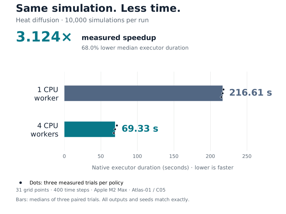
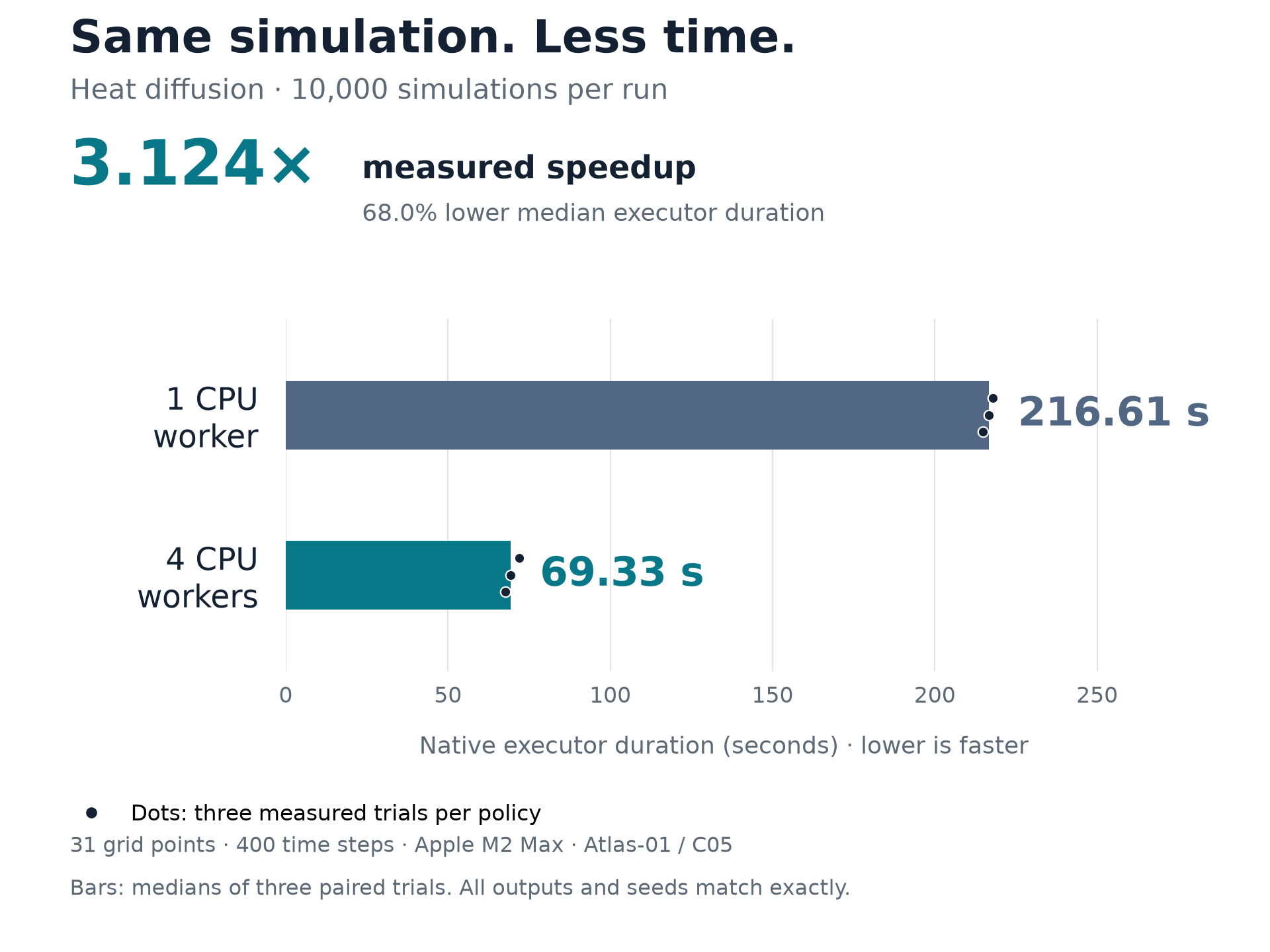
Bars start at zero and show median executor seconds across three paired trials: 216.606457 s with one worker and 69.327489 s with four. Dots mark each individual trial. Both worker policies use the same model, initial parameters and master seed. Each pair runs both ensembles sequentially in one process and verifies all 40,000 output cells and 10,000 derived seeds exactly. The observed 3.124× speedup corresponds to 68.0% lower median executor duration for this measured allocation, with the timing boundaries described below.
Download the vector SVG chart · Download the PNG chart
| Trial and execution order | One worker executor seconds | Four worker executor seconds | Paired executor speedup | Whole paired program wall seconds |
|---|---|---|---|---|
| 1: one then four | 214.909570 | 67.722272 | 3.173× | 282.667633 |
| 2: four then one | 216.606457 | 69.327489 | 3.124× | 285.973190 |
| 3: one then four | 217.792334 | 71.870100 | 3.030× | 289.716822 |
| Median times; ratio of medians | 216.606457 | 69.327489 | 3.124× | 285.973190 |
The ratio of median executor times is 3.124×, calculated as 216.606457 / 69.327489. Separately, the median of the three paired speedup ratios is 3.124×, with a measured range of 3.030× to 3.173×. These two summary definitions happen to agree for this record. Ratios are computed from unrounded measurements; displayed seconds are rounded to six decimals.
Every trial checked all 40,000 ordered output cells and all 10,000 derived seeds across worker counts, with zero mismatches. All four column means, sample variances and sample standard deviations also matched exactly within each pair and across the three trials. Native summaries confirm 10,000 completed iterations, four Float64 columns and peak active task counts of one and four. Each ensemble retained 320,000 numeric result bytes and reported 330,000 managed bytes including completion flags; interpreter/task heaps and process overhead are outside that result budget.
results.seconds() measures scheduling, per iteration parameter copying, task interpretation/output validation and row commits. It excludes context startup, initial admission/snapshot and final publication/statistics. Each whole paired program wall measurement includes both ensembles, parsing/checking, context setup, all cell/seed verification, statistics and printing. It is not the end to end latency of either worker policy alone. This measures scaling of checked Aner task execution in the native runtime, which interprets the task body. The observed speedup applies to this source, build, model and allocation; it is not a universal four worker speedup or physical model validation.
Reproduce and inspect the evidence
Use the website benchmark example or download the complete source. This is substantial CPU work: one normal invocation performs two 10,000 realization ensembles sequentially and requires at least four admitted CPU slots. It needs no external data, network, service or credential and creates no file.
aner check examples/parallel/repeat_heat_benchmark.aner
aner run examples/parallel/repeat_heat_benchmark.aner --max-steps 5000000
The published source sets let four_first = false. To reverse the execution order, change only that Bool to true; the model, input parameters, iteration count and master seed stay the same. The measured three trial order was false, true, false, after an excluded 100 realization per policy warm up. Preserve the explicit interpreter budget and record the source/build fingerprints when repeating the comparison. Four workers need four admitted CPU slots; parallel.inventory() reports the local policy.
Download the sanitized measured record for complete trials, native summaries, column statistics, timing boundaries and both median definitions. Its aner.heat-diffusion-benchmark/1 record retains public Atlas configuration identity and source/build content fingerprints, without private inventory, routes, credentials or runtime paths. SHA-256 values are content fingerprints, not digital signatures:
| Measured material | SHA-256 |
|---|---|
| Published benchmark source, one then four | cdec77431b6f05d35ca1e4ec597c5d3577b2df957251205a27223fa59b6dba67 |
| Reverse order source, only the Bool changed | 0e03c0c090ef8c6e5b0957ff6b7f41f998a0745b04f630e188da208db72dbbd8 |
Native executable, Atlas-01 / C05 | dfd628c32ee7a9c3feed1fb1a4498da5b9c66869daa52d420d33574f6d6c4f21 |
The record also retains the original heat source, warm up source and preserved model/configuration fingerprints. These checks distinguish measured numerical parity and execution scaling from the separate physical and numerical validation questions above.
Continue with the aner.parallel root guide, the repetition API, and the complete heat diffusion program.