Climate observations with retained evidence

This worked example uses actual NOAA NCEI daily observations, not simulated weather: Central Park, New York, station USW00094728, during leap year 2024. It demonstrates acquisition evidence, basic inspection, deliberate deep profiling, unit aware quality checks, immutable derived data, native charts and reproducibility checkpoints. It is descriptive exploration of one station year, not a climate trend or heatwave risk study.

Download the complete Aner program, normalized CSV, source manifest, preserved raw monthly records and station metadata, version marker and data notes. Keep the included relative folder tree when running the example:

aner check examples/climate_research.aner
aner run examples/climate_research.aner --display-dir climate-figures > climate-checkpoints.txt

Use fresh checkpoint/figure paths so earlier evidence remains intact; climate-figures must not already exist, and its parent must already exist. In the development VS Code extension, Run File opens the four figures beside the source. Execution is offline and needs no map pack, cloud account or Python runtime. The optional raw to CSV verification tool uses Python only when explicitly invoked.

Follow the evidence through the workflow

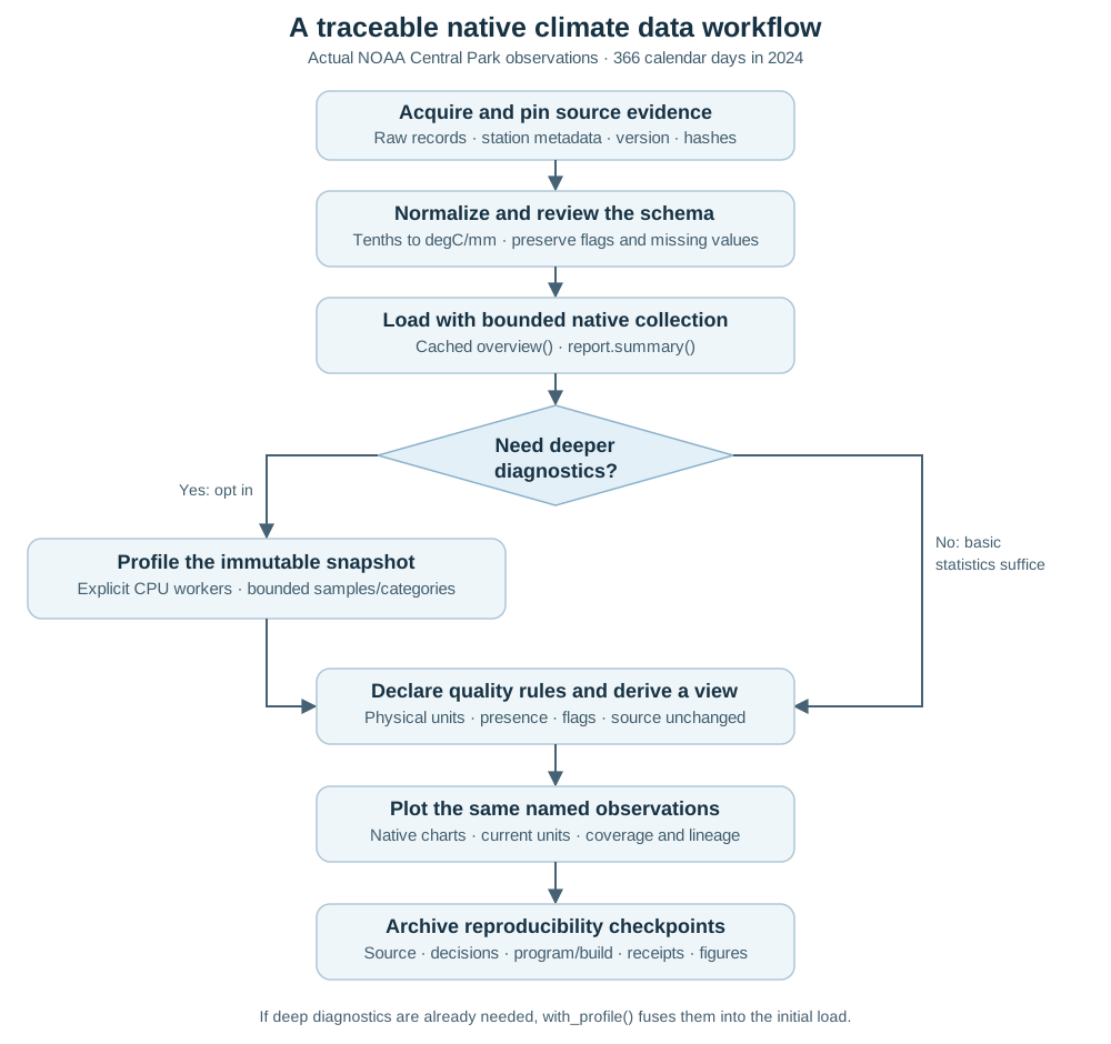
Download the standalone SVG workflow diagram.

If richer diagnostics are known to be needed before loading, put with_profile on the initial scan. It fuses their accumulation into collection. The example instead starts with inexpensive cached inspection and deliberately chooses one deeper traversal of the retained snapshot. overview() retrieves the cached report, and summary() formats it; neither hides a new source read.

Acquire a fixed source, then interpret its meaning

The NOAA GHCN Daily product integrates daily station records and can revise historical observations. The pinned manifest therefore records original byte identities and the retrieved version marker; the example does not download today's values every time it runs. Credit Menne and colleagues, GHCN Daily Version 3, NOAA NCDC, dataset DOI, accessed October 23, 2026, and the methods overview.

The offline replay converter expands the preserved monthly records into valid calendar days and applies the documented source scale/flag conventions. It preserves blank flags as empty Strings and missing values as NA; it does not fill gaps or discard flagged observations. Dates label daily observation periods. The program keeps them as Strings rather than inventing UTC midnight instants or assuming an undocumented timezone/observation window.

The manifest explicitly declares the upstream selection: one station, one year and three elements. A complete read of this CSV establishes completeness of the supplied snapshot, not acquisition of every NOAA record. The original station metadata, raw month lines and reproducible conversion remain beside the analysis.

Start with basic inspection

let source = data.scan_csv_auto("examples/fixtures/climate_noaa_2024/observations.csv",
    missing: "NA", memory_bytes: 8388608, sample_rows: 0)
let observations = source.collect(0, 8388608, 64)
let basic = observations.overview()
print(basic.summary())
print(basic.unit_mean("TMAX_DegC", "degC"))

overview() returns the cached structured DataReport with structure, missing counts, moments and extrema. Its summary() formats those together with storage and coverage; typed accessors retain physical context. These are available after ordinary collection. They add bounded per column accumulator work during loading, not dictionaries, distribution samples or another traversal. Basic statistics are not free CPU operations, and Float64 moments remain approximate floating point calculations. Identifier/date-code means printed by a type based summary are not climate measurements; field roles and scientific interpretation still require review.

Schema inference is a separate inspection pass. The example inspects the complete small input, then loads and validates it. An unfamiliar large source may use an advisory sample and reviewed schema overrides instead. Registered _DegC and _mm suffixes make the two temperature Points and precipitation Quantity explicit. Inspecting a date label does not make it a timestamp.

The pinned input contains 366 rows and no missing TMAX/TMIN/PRCP values. That is a finding about this snapshot, not evidence that real climate data never contain gaps. Aner's synthetic tests separately exercise missing and malformed observations; this government data example does not inject fake faults.

Choose deeper diagnostics deliberately

let deep = observations.select(List("TMAX_DegC", "TMIN_DegC", "PRCP_mm", "PRCP_mflag"))
    .with_profile_workers(4)
    .profile(max_bytes: 8388608, batch_rows: 64,
        sample_rows: 512, max_categories: 32)
print(deep.summary())
print(deep.quantile_text("TMAX_DegC", q: 0.5))

The example explicitly requests four native CPU workers for its four projected fields and checks deep.profile_workers(). One worker remains the default; a tiny station year can lose time to synchronization. Fused loading, parsing and validation remain serial. The measured cost guide documents resource admission and workload specific results, without claiming an automatic speedup.

The 512 value bound retains all 366 present temperatures, so the nearest rank quantiles are exact for this observed population. Its 50th percentile is 18.9 degC. This is not an interpolated median or a climatological normal. Larger populations expose sample counts and approximation flags; per column samples cannot be zipped into aligned observations.

For a future run where deep diagnostics are already desired, load once with source.with_profile(512, 32).collect(...), then retrieve table.profile() without an additional traversal. Ordinary table.profile() rejects uncaptured deep state; it never silently starts an expensive pass. The profiling guide defines bounded sampling, category overflow, exactness and resource controls.

Declare quality decisions and retain the source

let quality_clear = (data.col("TMAX_qflag") == "") &&
    (data.col("TMIN_qflag") == "") && (data.col("PRCP_qflag") == "")
let present = data.col("TMAX_DegC").is_present() &&
    data.col("TMIN_DegC").is_present() && data.col("PRCP_mm").is_present()
let physically_ordered = (data.col("TMAX_DegC") >= data.col("TMIN_DegC")) &&
    (data.col("PRCP_mm") >= 0.0@mm)
let accepted = observations.filter(quality_clear && present && physically_ordered)
    .collect(0, 8388608, 64)
let warm = accepted.filter(data.col("TMAX_DegC") >= 30.0@degC)
    .select(List("observation_id", "date", "TMAX_DegC", "PRCP_mm"))
    .collect(0, 8388608, 64)

All 366 supplied rows pass these declared checks; the threshold screen selects 39. The raw table remains unchanged. A blank quality flag records that the listed source checks did not fail; it does not prove perfect measurement. The comparison uses compatible physical Point/Quantity meanings, and no bare numeric threshold silently acquires a temperature unit.

The sample includes 44 trace precipitation flags whose recorded numeric total is zero, and 125 days with positive recorded precipitation. Trace remains trace. The program does not replace missing precipitation with zero, relabel every zero as a dry day, or treat 30 degC as a validated heatwave definition. A study specific event definition needs an appropriate baseline, duration rule and scientific rationale.

Plot the same named observations

let seasonal = plot.scatter(accepted,
    x: "day_of_year", y: "TMAX_DegC", max_points: 366)
let distribution = plot.distribution(deep, "TMAX_DegC", bins: 18)
let paired = plot.scatter(accepted,
    x: "TMIN_DegC", y: "TMAX_DegC", max_points: 366)
seasonal.show()

All 366 source rows are inspected. Day of year is an explicitly derived coordinate for this leap year, not an invented UTC timestamp. The seasonal pattern is visible; the figure does not fit or establish a long term trend.

This histogram contains all observed daily maxima because the bound exceeds the population. In a larger sampled profile, its caption and structured lineage disclose the sample policy instead of inflating sample bin counts into population totals.

The paired plot uses same row table coordinates. It does not combine independently sampled profile columns or claim an inferential correlation result. The example additionally produces a missingness chart, confirming zero missing values in the four profiled fields.

Every adapter carries current units, coverage and immutable construction lineage into native SVG/HTML metadata. Derived table source recipes retain parent logical identities and input-kind/digest links, so the original supplied CSV hash remains reachable through recursive parent recipes without retaining parent payloads or volatile timing receipts. Formatting edits do not turn that lineage into a complete audit of later manual changes. Retain both the program and exported figure. The plotting guide defines chart bounds and the distinction between numerical coordinate limits and exact scientific data storage.

Freeze checkpoints before interpreting results

The example prints raw/derived provenance, deep profile JSON, runtime/build identification and chart provenance. Archive that stdout with the source CSV, raw monthly records, station metadata, manifest, conversion script and analysis program. The normalized CSV's pinned SHA-256 is 96d02e4aa0e083e50e5283ba6b06fc95d15992c666e78496e3aff45351a211e7. Independent conversion checks and the executable example test verify population counts and source identities.

complete concerns the immediate terminal. origin_complete additionally preserves known ancestry: profiling an entire seven row preview snapshot can be complete while its origin remains incomplete. Repeated collection cannot validate the unread original tail. Neither flag discovers upstream records omitted before a source was supplied; the acquisition manifest supplies that separate evidence.

One station year does not establish long term warming, a regional climate estimate, causal effects, independent daily observations or city wide heat exposure. Climate research needs appropriate long/homogeneous records, station history and coverage assessment, observation window rules, justified aggregation and uncertainty modeling. A predictive extension must split by the appropriate time/group unit and learn preprocessing from training observations alone. Native receipts and physical types support those decisions; they do not make them automatically correct.

See the Native data processing module reference for the shared API.